Julia is a feature-rich language. It was designed to appeal to novice programmers and purists alike. For those whose interests lie in data science, statistics, and mathematical modeling, Julia is well-equipped to meet all their needs.

Our aim is to furnish you with the necessary knowledge to begin programming in Julia almost immediately. So, rather than begin with an overview of the language’s syntax, control structures, and the like, we will introduce Julia’s facets gradually over the rest of this book. Over the next four chapters, we will look at some of the basic and advanced features of the Julia core. Many of the features—such as graphics and database access, which are implemented via the package system—will be left until later when discussing more specific aspects of programming Julia.

In this chapter, we will be discussing manipulating Julia’s data structures and will cover the following topics:

• Data types such as integers and floating-point and complex numbers
• Vectors, matrices, and multi-dimensional arrays
• List comprehensions and broadcasting
• Recursive functions
• Characters and strings
• Complex and rational numbers
• Data arrays and data frames
• Dictionaries, sets, stacks, and queues

If you are familiar with programming in Python, R, MATLAB, and so on, you will not find the journey terribly arduous; in fact, we believe it will be a particularly pleasant one.

All code files are placed on GitHub at https://github.com/PacktPublishing/Mastering-Julia-Second-Edition. Refer to the section in the Preface for details on how to download and run them.

While Julia is usually dynamically typed—that is, in common with most interpreted languages, it does not require the type to be specified when a variable is declared; rather, it infers it from the form of the declaration. However, it also can be considered as a strongly typed language and, in this case, allows the programmer to specify a variable’s type precisely.

A variable in Julia is any combination of upper- or lowercase letters, digits, and the underscore (_) and exclamation (!) characters. It must start with a letter or an underscore.

Conventionally, variable names consist of lowercase letters with long names separated by underscores rather than using camel case.

To determine a variable type, we can use the typeof() function, as follows:

julia> x = 2;   typeof(x) # => gives Int
julia> x = 2.0; typeof(x) # => gives Float

Notice that the type (see the preceding code) starts with a capital letter and ends with a number, which indicates the number of bit length of the variable. The bit length defaults to the word length of the operating system, and this can be determined by examining the WORD_SIZE built-in constant, as follows:

julia> WORD_SIZE # => 64 (on my MacPro computer)

In this section, we will be dealing first with integer and Boolean types.

Integers

An integer type can be any of Int8, Int16, Int32, Int64, and Int128, so the maximum integer can occupy 16 bytes of storage and be anywhere within the range of –2127 to (+2127 - 1).

If we need more precision than this, Julia core implements the BigInt type:

julia> x = BigInt(2^32)
6277101735386680763835789423207666416102355444464034512896

As well as the integer type, Julia provides the unsigned integer type, UInt; again, UInt ranges from 8 to 128 bytes, so the maximum UInt value is (2128 - 1).

We can use the typemax() and typemax() functions to output the ranges of the Int and UInt types, like so:

julia> for T =
  Any[Int8,Int16,Int32,Int64,Int128,UInt8,UInt16,UInt32,UInt64,UInt128]
  println("$(lpad(T,7)): [$(typemin(T)),$(typemax(T))]")
end
Int8: [-128,127]
Int16: [-32768,32767]
Int32: [-2147483648,2147483647]
Int64: [-9223372036854775808,9223372036854775807]
Int128: [-170141183460469231731687303715884105728,
          170141183460469231731687303715884105727]
UInt8: [0, 255]
UInt16: [0, 65535]
UInt32: [0, 4294967295]
UInt64: [0, 18446744073709551615]
UInt128: [0, 340282366920938463463374607431768211455]

Particularly, notice the use of the form of the for statement, which we will discuss when we deal with arrays and matrices later in this chapter.

Suppose we type the following:

julia> x = 2^32; x*x # => the answer 0

The reason for the answer being 0 is that the integer “wraps” around, so squaring 232 gives 0, not 264, since my WORD_SIZE value is 64:

julia> x = int128(2^32); x*x
# => the answer we would expect 18446744073709551616

We can use the typeof() function on a type such as Int64 in order to see what its parent type is:

# So typeof(Int64) gives DataType and typeof(UInt128) also gives DataType.

A definition of DataType is hinted at in the boot.jl core file; I say hinted at because the actual definition is implemented in C, and the Julia equivalent is commented out.

Definitions of the integer types can also be found in boot.jl, this time not commented out.

In the next chapter, we will discuss the Julia type system in some detail. Here, it is worth noting that we distinguish between two kinds of data types: abstract and primitive (concrete).

The general syntax for declaring an abstract type is shown here:

abstract type «name» end
abstract type «name» <: «supertype» end

Typically, this is how it would look:

abstract type Number end
abstract type Real <: Number end
abstract type AbstractFloat <: Real end
abstract type Integer <: Real end
abstract type Signed <: Integer end
abstract type Unsigned <: Integer end

Here, the <: operator corresponds to a subclass of the parent.

Let’s suppose we type the following:

julia> x = 7; y = 5; x/y # => this gives 1.4

Here, the division of two integers produces a real result. In interactive mode, we can use the ans symbol to correspond to the last answer—that is, typeof(ans) gives Float.

To get the integer divisor, we use the div(x,y) function, which gives 1, as expected, and typeof(ans) is Int64. The remainder is obtained either by rem(x,y) or by using the % operator.

Julia has one curious operator—the backslash. Syntactically, x\y is equivalent to y/x. So, with x and y, as before, x\y gives 0.71428 (to 5 decimal places).

Primitive types

A primitive type is a concrete type whose data consists of a series of bits. Examples of primitive types are the (well-known) integers and floating-point values that we have met previously.

The general syntax for declaring a primitive type is like that of an abstract type but with the addition of the number of bits to be allocated:

primitive type «name» «bits» end
primitive type «name» <: «supertype» «bits» end

Since Julia is written (mostly) in Julia, a corollary is that Julia lets you declare your own primitive types, rather than providing only a fixed set of built-in ones.

That is, all the standard primitive types are defined in Base itself, as follows:

primitive type Float16 <: AbstractFloat 16 end
primitive type Float32 <: AbstractFloat 32 end
primitive type Float64 <: AbstractFloat 64 end
primitive type Bool <: Integer 8 end
primitive type Char 32 end
primitive type Int8 <: Signed 8 end
primitive type UInt8 <: Unsigned 8 end
primitive type Int16 <: Signed 16 end
primitive type UInt16 <: Unsigned 16 end
primitive type Int32 <: Signed 32 end
primitive type UInt32 <: Unsigned 32 end
primitive type Int64 <: Signed 64 end
primitive type UInt64 <: Unsigned 64 end
primitive type Int128 <: Signed 128 end
primitive type UInt128 <: Unsigned 128 end

Note that only sizes that are multiples of 8 bits are supported, so Boolean values, although they really need just a single bit, cannot be declared to be any smaller than 8 bits. Figure 2.1 demonstrates a portion of the Julia hierarchical structure as it applies to simple numerical types:

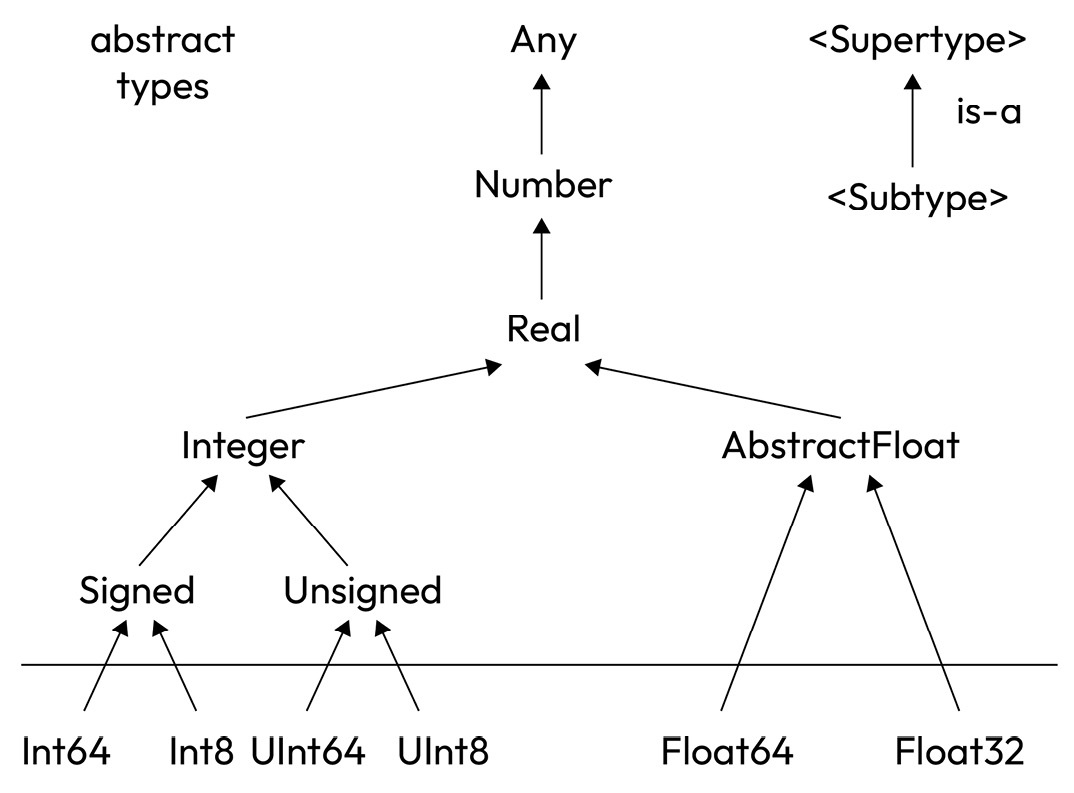
Figure 2.1 – Tree structure for numerical types

Those above the line are abstract types beginning with Any and cascading down through Number and Real before splitting into Integer and AbstractFloat types, eventually reaching the primitive types defined in Julia Base, which are shown below the line.

Primitives can’t be subclassed further, hence terminating the various branches of the tree.

Logical and arithmetic operators

As well as decimal arguments it is possible to assign binary, octal, and hexadecimal ones using the 0b, 0o, and 0x prefixes.

So, x = 0b110101 creates the hexadecimal number 0x35 (that is, decimal 53), and typeof(ans) is UInt8 since 53 will “fit” into a single byte.

For larger values, the type is correspondingly higher—that is, x = 0b1000010110101 gives x = 0x10b5, and typeof(ans) is UInt.

When operating on bits, Julia provides ~ (not), | (or), & (and), and $ (xor):

julia> x = 0xbb31;  y = 0xaa5f;
julia> x$y
0x116e

Also, we can perform arithmetic shifts using the (LEFT) and (RIGHT) operators.

Note

Because x is of the UInt16 type, the shift operator retains that size, so x = 0xbb31; x<<8. This gives 0x3100 (the top two nibbles being discarded), and typeof(ans) is UInt.

Booleans

Julia has the Bool logical type. Dynamically, a variable is assigned a Bool type by equating it to the true or false constant (both lowercase), or alternatively, to a logical expression such as the following:

julia> p = (2 < 3) # => true
julia> typeof(p)   # => Bool

Many languages treat 0, empty strings, and NULL instances as representing false and anything else as true. This is NOT the case in Julia, however; there are cases where a Bool value may be promoted to an integer, in which case true corresponds to unity.

That is, an expression such as x + p (where x is of the Int type and p of the Bool type) will output the following:

julia> x = 0xbb31; p = (2 < 3);
julia> x + p
0xbb32
julia> typeof(ans) # => UInt16

Big integers

Let’s consider the factorial function defined by the usual recursive relation:

# n! = n*(n-1)! for integer values of n (> 0)
function fac(n::Integer)
  @assert n > 0
  (n == 1) ? 1 : n*fac(n-1)
end

Note that since normally, integers in Julia overflow (a feature of Low-Level Virtual Machine (LLVM), the preceding definition can lead to problems with large values of n, as illustrated here:

julia> using Printf
       for i = 20:30
         @printf "%3d : %d\n" i fac(i)
       end
 20 : 2432902008176640000
 21 : -4249290049419214848
 22 : -1250660718674968576
 23 : 8128291617894825984
 24 : -7835185981329244160
 25 : 7034535277573963776
 26 : -1569523520172457984
 27 : -5483646897237262336
 28 : -5968160532966932480
 29 : -7055958792655077376
 30 : -8764578968847253504
# Since a BigInt <: Integer,
# if we pass a BigInt the routine returns the correct value
julia> fac(big(30))
265252859812191058636308480000000
# See can check this since integer values: Γ(n+1) === n!
julia> gamma(31)
2.6525285981219107e32

The big() function uses string arithmetic, so it does not have a limit imposed by the WORD_SIZE constant but is clearly much slower than using conventional arithmetic. The big() function is not only restricted to integers but can be applied to reals (floats) or even complex numbers.

We can introduce a new function, |>, which applies a function to its preceding argument, providing a chaining functional style:

julia> 30 |> big |> fac
265252859812191058636308480000000

Here, the 30 argument is piped to the factorial function but after first being converted into a BigInt type.

Also, note that the syntax is equivalent to fac(big(30)).

For now, we are going to leave our discussion on functions and begin to study in depth how arrays are constructed and used in Julia.

An array is an indexable collection of (normally) heterogeneous values such as integers, floats, and Booleans. In Julia, unlike many programming languages, the index starts at 1, not 0.

One-dimensional arrays are also termed vectors and two-dimensional arrays as matrices.

Let’s define the following vector:

julia> A = [1, 1, 2, 3, 5, 8, 13, 21, 34, 55, 89, 144, 233, 377, 
610];
julia> typeof(A)
Vector{Int64} (alias for Array{Int64, 1})

This represents a column array, whereas not using the comma as an element separator creates a row matrix:

julia> A = [1 1 2 3 5 8 13 21 34 55 89 144 233 377 610];
julia> typeof(A)
Matrix{Int64} (alias for Array{Int64, 2})

We observed these are the first 15 numbers of the well-known Fibonacci sequence.

In conjunction with loops in the Asian option example in the previous chapter, we meet the definition of a range as start:[step]:end:

julia> A = 1:10; typeof(A)
UnitRange{Int64}
julia> B = 1:3:15; typeof(B)
StepRange{Int64,Int64}
julia> C = 0.0:0.2:1.0; typeof(C)
StepRangeLen{Float64,Base.TwicePrecision{Float64},
                     Base.TwicePrecision{Float64}, Int64}

In Julia, the preceding definition returns a range type.

To convert a range to an array, we have seen previously that it is possible to use the collect() function, as follows:

julia> C = 0.0:0.2:1.0; collect(C)
6-element Vector{Float64}:
0.0
0.2
0.4
0.6
0.8
1.0

Julia also provides functions such as zeros(), ones(), and rand(), which provide array results.

Normally, these functions return floating-point values, so a little bit of TLC is needed to provide integer results, as seen in the following code snippet:

A = convert.(Int64,zeros(15));
B = convert.(Int64,ones(15));
C = convert.(Int64,rand(1:100,15));

The preceding code is an example of broadcasting in Julia, and we will discuss it a little further in the next section.

Broadcasting and list comprehensions

Originally, the application of operators to members of an array was implemented using a broadcast() function. This led to some pretty unwieldy expressions, so this was simplified by the preceding “dot” notation.

Let’s define a 2x3 matrix of rational numbers and convert them to floats, outputting the result to 4 significant places:

julia> X = convert.(Float64, [11/17 2//9 3//7; 4//13 5//11 6//23])
2×3 Matrix{Float64}:
 0.647059  0.222222  0.428571
 0.307692  0.454545  0.26087
julia> round.(X, digits=4)
2×3 Matrix{Float64}:
 0.6471  0.2222  0.4286
 0.3077  0.4545  0.2609

Note that the second statement does not alter the actual precision of the values in X unless we reassign—that is, X = round,(X, digits=4).

Consider the function we plotted in Chapter 1 to demonstrate the use of the UnicodePlots package:

julia> f(x) = x*sin(3.0x)*exp(-0.03x)

This does not work when applied to the matrix, as we can see here:

julia> Y = f(X)
ERROR: Dimension Mismatch: matrix is not square: dimensions are (2, 3)

But it can be evaluated by broadcasting; in this case, the broadcasting dot follows the function names, and also note that broadcasting can be applied to a function defined by ourselves, not just to built-in functions and operators:

julia> Y = f.(X)
2×3 Matrix{Float64}:
 0.591586  0.136502  0.40602
 0.243118  0.438802  0.182513

This can also be done without the f() temporary function:

julia> Y = X .* sin.(3.0 .* X) .* exp.(- 0.03 .* X)
2×3 Matrix{Float64}:
 0.591586  0.136502  0.40602
 0.243118  0.438802  0.182513

Finally, in the following example, we are using the |> operator we met previously and an anonymous function:

julia> X |> (x -> x .* sin.(3.0 .* x) .* exp.(- 0.03 .* x))
2×3 Matrix{Float64}:
 0.591586  0.136502  0.40602
 0.243118  0.438802  0.182513

This introduces the alternate style (x -> f(x)) as a mapping function, equivalent to the syntax to map (f,X).

Another method of creating and populating an array is by using a list comprehension:

# Using a list comprehension is a bit more cumbersome
julia> Y = zeros(2,3);
julia> [Y[i,j] =
        X[i,j]*sin(3.0*X[i,j])*exp(-0.03*X[i,j]) for i=1:2 for j=1:3];
julia> Y
2×3 Matrix{Float64}:
 0.591586  0.136502  0.40602
 0.243118  0.438802  0.182513

There are cases where a list comprehension is useful—for example, to list only odd values of the Fibonacci series, we can use the following statement:

julia> [fac(k) for k in 1:9 if k%2 != 0]
5-element Vector{BigInt}:
      1
      6
    120
   5040
 362880

For the moment, armed with the use of arrays, we will look at recursion and how this is implemented in Julia.

We considered previously the factorial function, which was an example of a function that used recursion—that is, it called itself. Recursive definitions need to provide a way to exit from the function. Intermediate values are pushed on the stack, and on exiting, the function unwinds, which has the side effect that a function can run out of memory, and so is not always the best (or quickest) method of implementation.

An example in the previous section where this is the case is computing values in the Fibonacci sequence, and we explicitly enumerate the first 15 values. Let’s look at this in a bit more detail:

• The series has been identified as early 200 BCE by Indian mathematician Pingala.
• More recently, in Europe around 1200, Leonardo of Pisa (aka Fibonacci) posed the problem of an idealized rabbit population, where a newly born breeding pair of rabbits are put out together and each breeding pair mates at the age of 1 month. At the end of the second month, they produce another pair of rabbits, and the rabbits never die. Fibonacci considered the following question: How many pairs will there be in 1 year?
• In nature, the nautilus shell chambers adhere to the Fibonacci sequence’s logarithmic spiral, and this famous pattern also shows up in many areas, such as flower petals, pinecones, hurricanes, and spiral galaxies.

We noted that the sequence can be defined by the recurrence relation, as follows:

julia> A = Array{Int64}(undef,15);
julia> A[1]=1; A[2]=1;
julia> [A[i] = A[i-1] + A[i-2] for i = 3:length(A)];

This presents a similar problem to the factorial in as much as eventually, the value of the Fibonacci sequence will overflow.

To code this in Julia is straightforward:

function fib(n::Integer)
  @assert n >= 1
  return (n == 1 || n == 2 ? 1 : (fib(n-1) + fib(n-2)));
end

So, the answer to Fibonacci’s problem is fib(12), which is 144.

A more immediate problem is with the recurrence relation itself, which involves two previous terms, and the execution speed will get rapidly (as 2n ) longer.

My Mac Pro (Intel i7 processor with 16 GB RAM) runs out of steam around the value 50:

julia> @time fib(50);
 75.447579 seconds

To avoid the recursion relation, a better version is to store all the intermediate values (up to n) in an array, like so:

function fib1(n::Integer)
  @assert n > 0
  a = Array{typeof(n),1}(undef,n)
  a[1] = 1
  a[2] = 1
  for i = 3:n
    a[i] = a[i-1] + a[i-2]
  end
  return a[n]
end

Using the big() function avoids overflow problems and long runtimes, so let’s try a larger number:

julia> @time(fib1(big(101)))
0.053447 seconds (115.25 k allocations: 2.241 MiB)
573147844013817084101

A still better version is to scrap the array itself, which reduces the storage requirements a little, although there is little difference in execution times:

function fib2(n::Integer)
  @assert n > 0
  (a, b) = (big(0), big(1))
  while n > 0
    (a, b) = (b, a+b)
  n -= 1
  end
  return a
end
julia> @time(fib2(big(101)))
0.011516 seconds (31.83 k allocations: 760.443 KiB)
573147844013817084101

Observe that we need to be careful about our function definition when using list comprehensions or applying the |> operator.

Consider the following two definitions of the Fibonacci sequence we gave previously:

julia> [fib1(k) for k in 1:2:9 if k%2 != 0]
ERROR: BoundsError:attempt to access 1-element Vector{Int64} at index 
[2]
julia> [fib2(k) for k in 1:2:9 if k%2 != 0]
5-element Vector{BigInt}:
  1
  2
  5
 13
 34

The first version, which uses an array, raises a bounds error when trying to compute the first term, fib1(1), whereas the second executes successfully.

Implicit and explicit typing

In the definitions and the factorial function and Fibonacci sequence, the type of the input parameter was explicitly given (as an integer), which allowed Julia to raise that an error is real, complex, and so on, and was passed. This allowed us to check for positivity using the @asset macro.

The question arises: Can the return type of a function be specified as well? The answer is yes.

Consider the following code, which computes the square of an integer. The return value is a real number (viz. Float64) where normally, we would have expected an integer; we term this process as promotion, which we will discuss in more detail later in the book:

julia> sqi(k::Integer)::Float64 = k*k
sqi (generic function with 1 method)
julia> sqi(3)
9.0

In the next example, the input value is taken as a real number but the return is an integer:

julia> sqf(x::Float64)::Int64 = x*x
sqf (generic function with 1 method)

This works when the input can be converted exactly to an integer but raises an InexactError error otherwise:

julia> sqf(2.0)
4
julia> sqf(2.3)
ERROR: InexactError: Int64(5.289999999999999)

Alternatively, let’s consider explicitly specifying the type of a variable.

When using implicit typing, the variable can be reassigned and its type changes appropriately:

julia> x = 2; typeof(x)
Int64
julia> x = 2.3; typeof(x)
Float64
julia> x = "Hi"; typeof(x)
String

Now, if we try to explicitly define the type of the existing variable, it raises an error:

julia> x::Int64 = 2; typeof(x)
ERROR: cannot set type for global x. It already has a value or is 
already set to a different type.

So, let’s start with a new as yet undefined variable:

julia> y::Int64 = 2; # => 4
julia> typeof(y)
Int64

In this case, assigning the input to a non-integer results in an InexactError error, as before:

julia> y = 2.3
ERROR: InexactError: Int64(2.3)

Also, we cannot redefine the type of the variable now it has been defined:

julia> y::Float64 = 2.3; typeof(y)
ERROR: cannot set type for global y. It already has a value or is 
already set to a different type.

Finally, suppose that we prefix the assignment with the local epithet; this seems to be OK except that the variable type is unchanged and its value rounded down rather than an error being raised:

julia> local y::Float64 = 2.3;
julia> typeof(y)
Int64
julia> y
2

The value of the y global is not changed since we are not introducing a new block, and so the scope remains the same.

So far, we have been discussing arrays consisting of a single index (aka one-dimensional), which are equivalent to vectors. In fact, only column-wise arrays are considered to be vectors—that is, consisting of a single column and multiple rows. Here’s an example:

julia> [1; 2; 3]
3-element Vector{Int64}:
 1
 2
 3

Alternatively, an array comprising a single row and multiple columns is viewed as a two-dimensional array, which is commonly referred to as a matrix. We will turn to operating on matrices next:

julia> [1 2 3]
1×3 Matrix{Int64}:
 1  2  3

Note that a vector is created by separating individual items using a semicolon, whereas the 1x3 matrix is constructed only as space(s). This convention is used in creating multirow and column arrays.

We will be meeting matrices and matrix operations throughout this book, but let us look now at the simplest of operations.

Let’s take A and B, as defined in the following code snippet:

julia> A = [1 2 3; 4 5 6];
julia> B = [1 5; 4 3; 2 6];

The normal matrix rules apply, which is a feature of multiple dispatch; we will cover this in Chapter 4.

The transpose of B can be computed as follows:

julia> C = transpose(B)
2×3 transpose(::Matrix{Int64}) with eltype Int64
1 4 2
5 3 6

This can also be written more compactly as C = B’:

julia> A + C
2x3 Matrix{Int64}:
2 6 5
9 8 12
julia> A*B
2x2 Matrix{Int64}:
15 29
36 71

Matrix division makes more sense with square matrices, but it is possible to define the operations for non-square matrices too. Note here that the / and \ operations produce results of different sizes:

julia> A / C
2x2 Matrix{Float64}
0.332273 0.27663
0.732909 0.710652
julia> A \ C
3x3 Matrix{Float64}:
 1.27778  -2.44444  0.777778
 0.444444 -0.111111 0.444444
-0.388889  2.22222  0.111111

The type of the array was previously defined as Array{Int64,2} rather than the now more compact form of Matrix{Int64}, and ditto Array{Float64,2} has been replaced with Matrix{Float64}.

We will discuss matrix decomposition in more detail later when looking at linear algebra.

Although A * C is not allowed because the number of columns of A is not equal to the number of rows of C, the following broadcasts are all valid:

julia> A .* C 2x3 Matrix{Int64}: 1  8  6 20 15 36
julia> A ./ C 2x3 Matrix{Float64}: 1.0 0.5     1.5 0.8 1.66667 1.0
julia> A .== C 2x3 BitMatrix 1  0  0 0  0  1

So far, we have only been looking at manipulating variables representing arithmetic values. Julia has a variety of string types, which we will look at next.

The simplest character-based variables consist of ASCII and Unicode characters.

A single character is delimited by single quotes, whereas a string uses double quotes or, in some cases, triple-double quotes (“””), which is discussed in this section.

A string can be viewed as a one-dimensional array of characters and can be indexed and manipulated in a similar fashion as an array of numeric values:

julia> s = "Hi there, Blue Eyes!"
"Hi there, Blue Eyes!"
julia> length(s)
20
julia> s[11]
'B': ASCII/Unicode U+0042 (category Lu: Letter, uppercase)
julia> s[end]
'!': ASCII/Unicode U+0021 (category Po: Punctuation, other)

Hint—Try evaluating the following list comprehension: [s[i] for i = length(s):-1:1].

Characters

Observe that Julia has a built-in Char type to represent a character.

A character occupies 32 bits, not 8, which is why it can hold a Unicode character. Have a look at the following example:

# All the following represent the ASCII character capital-A
julia> c = 'A';
julia> c = Char(65);
julia> c = '\U0041'
'A': ASCII/Unicode U+0041 (category Lu: Letter, uppercase)

Julia supports Unicode code, as we see here:

julia> c = '\Uc041'
'': Unicode U+c041 (category Lo: Letter, other)

As such, we can output characters from a variety of different alphabets—for example, Chinese:

 julia> '\U7537'
'男': Unicode U+7537 (category Lo: Letter, other)

It is possible to specify a character code of '\Uffff' but char conversion does not check that every value is valid. However, Julia provides an isvalid() function that can be applied to characters:

julia> c = '\Udff3'; isvalid(c)
false

Julia uses the special C-like syntax for certain ASCII control characters such as '\b', '\t', '\n', '\r', and 'f' for backspace, tab, newline, carriage-return, and form-feed, respectively.

The backslash acts as an escape character, so Int('\s') => 115, whereas Int('\t') => 9.

If more than one character is supplied between the single quotes, this raises an error:

julia> 'Hello'
ERROR: syntax: character literal contains multiple characters

Strings

The type of string we are most familiar with comprises a list of ASCII characters that, as we have observed, are normally delimited with double quotes, as in the following example:

julia> s = "Hello there, Blue Eyes";
julia> typeof(s)
String

The following points are worth noting:

• The built-in concrete type used for strings (and string literals) is String
• This supports the full range of Unicode characters via UTF-8 encoding
• All string types are subtypes of the AbstractString abstract type, so when defining a function expecting a string argument, you should declare the type as AbstractString in order to accept any string type

A transcode() function can be used to convert to/from other Unicode encodings:

julia> s = "αβγ";
julia> transcode(UInt16, s)
3-element Vector{UInt16}:
 0x03b1
 0x03b2
 0x03b3

In Julia (as in Java), strings are immutable—that is, the value of a String object cannot be changed. To construct a different string value, you construct a new string from parts of other strings. Let’s look at this in more detail:

• ASCII strings are indexable, so from s as defined previously: s[14:17] # => "Blue".
• The values in the range are inclusive, and if we wish, we can change the increment to s[14:2:17] => "Bu" or reverse the slice to s[17:–1:14] => "eulB".
• Omitting the end of the range is equivalent to running to the end of the string: s[14:] => "Blue Eyes".
• However, s[:14] is somewhat unexpected and gives the character 'B', not the string up to and including B. This is because ':' defines a “symbol”, and for a literal, :14 is equivalent to 14, so s[:14] is the same as s[14] and not s[1:14].
• The final character in a string can be indexed using the notation end, so in this case, s[end] is equal to the 's' character.

Strings allow for special characters such as \n, \t, and so on.

If we wish to include the double quotes, we can escape them, but Julia provides a """ delimiter.

So, s = "This is the double quote \" character" and s = """This is the double quote " character""" are equivalent:

julia> s = "This is a double quote \" character."; println(s);
This is a double quote " character.

Strings also provide the “$" convention when displaying the value of a variable:

julia> age = 21; s = "I've been $age for many years now!"
I've been 21 for many years now!

Concatenation of strings can be done using the $ convention, but Julia also uses the '*' operator (rather than '+' or some other symbol):

julia> s = "Who are you?";
julia> t = " said the Caterpillar."
julia> s*t or "$s$t" # => "Who are you? said the Caterpillar."

Note

Here’s how a Unicode string can be formed by concatenating a series of characters:

julia> '\U7537'*'\U4EBA'

“男人’’

Regular expressions

Regular expressions (regexes) came to prominence with their inclusion in Perl programming.

There is an old Perl programmer’s adage: “I had a problem and decided to solve it using regular expressions; now, I have two problems.”

Regexes are used for pattern matching; numerous books have been written on them, and support is available in a variety of programming languages post-Perl, notably Java and Python. Julia supports regexes via a special form of string prefixed with r.

Suppose we define an empat pattern as follows:

julia> empat = r"^\S+@\S+\.\S+$"
julia> typeof(empat)
Regex

The following example will give a clue to what the pattern is associated with:

julia> occursin(empat, "fred.flintstone@bedrock.net")
true
julia> occursin(empat, "Fredrick Flintstone@bedrock.net")
false

The pattern is for a valid (simple) email address, and in the second case, the space in Fredrick Flintstone is not valid (because it contains a space!), so the match fails.

Since we may wish to know not only whether a string matches a certain pattern but also how it is matched, Julia has a match() function:

julia> m = match(r"@bedrock","barney,rubble@bedrock.net")
RegexMatch(„@bedrock")

If this matches, the function returns a RegexMatch object; otherwise, it returns Nothing:

julia> m.match
"@bedrock"
julia> m.offset
14
julia> m.captures
0-element Array{Union{Nothing,SubString{String}},1}

A detailed discussion of regexes is beyond the scope of this book.

The following link provides a good online source for all things regex, including an excellent cheat sheet via the Quick Reference page: https://www.rexegg.com.

In addition, there are a number of books on the subject, and a free PDF can be downloaded from the following link:

https://www.academia.edu/22080976/Regular_expressions_cookbook_2nd_edition.

Version strings

Version numbers can be expressed with non-standard string literals as v“…”.

These literals create VersionNumber objects that follow the specifications of “semantic versioning” and therefore are composed of major, minor, and patch numeric values, followed by pre-release and build alpha-numeric annotations.

So, a full specification typically would be “v1.9.1-rc1”, where the major version is “1”, minor version “9”, patch level “1”, and release candidate “1”.

Currently, only the major version needs to be provided, and the others will assume default values; for example, “v1” is equivalent to “v1.0.0”.

(The release candidate has no default, so needs to be explicitly defined.)

Byte array literals

Another special form is the b“…” byte array literal, which permits string notation to express arrays of UInt8 values.

These are the rules for byte array literals:

• ASCII characters and ASCII escape sequences produce a single byte
• \x and octal escape sequences produce a byte corresponding to the escape value
• Unicode escape sequences produce a sequence of bytes encoding that code points in UTF-8

Consider the following two examples:

julia> A = b"HEX:\xefcc"
7-element Base.CodeUnits{UInt8,String}:
[0x48,0x45,0x58,0x3a,0xef,0x63,0x63]
julia> B = b"\u2200 x \u2203 y"
11-element Base.CodeUnits{UInt8,String}:
0xe2
0x88
0x80
0x20
0x78
0x20
0xe2
0x88
0x83
0x20
0x79

Here, the first three elements represent the \u2200 code, then 0x20,0x78,0x20 correspond to <space>x<space>, followed by three more elements for the \u2203 code, and finally, 0x20, 0x79, which represents <space>y.

We have met the syntax for rational numbers in the previous chapter, and we will review operations on them here. Also, we will introduce another arithmetic type: complex numbers.

Complex numbers

There are two ways to define a complex number in Julia—first, using the Complex type definition as its associated Complex() constructor:

# Note the difference in these two definitions
julia> c = Complex(1, 2); typeof(c)
Complex{Int64}
julia> c = Complex(1, 2.0); typeof(c)Complex{Float64}
julia> c = ComplexF32(1,2.0); typeof(c)Complex{Float32}

Because in the second example, the complex number consists of an ordered pair of two reals, its size is 128 bits, whereas ComplexF32 has 2x Float32 arguments and ComplexF16 will have 2x Float16 arguments.

The Complex(0.0,1.0) number corresponds to the imaginary number 'I'—that is, sqrt(-1.0)—but Julia uses the 'im' symbol rather than 'I' to avoid confusion with an I variable, frequently used as an index iterator.

Hence, Complex(1, 2) is exactly equivalent to 1 + 2*im, but normally the '*' operator is omitted, and this would be expressed as 1 + 2im.

The complex number supports all normal arithmetic operations, as illustrated here:

julia> c = 1 + 2im;
julia> d = 3 + 4im;
julia> c*d
-5 + 10im
julia> c/d
0.44 + 0.08im
julia> c\d
2.2 - 0.4im

The c/d and c\d divisions produce real arguments even when the components are integers.

This is like Julia’s behavior with a simple division of integers. Also, it defines real(), imag(), conj(), abs(), and angle() complex functions.

abs and angle can be used to convert complex arguments to polar form:

julia> c = 1.0 + 2im; abs(c)
2.23606797749979
julia> angle(c)
1.1071487177940904 # (in radians)

Complex versions of many mathematical functions can be applied:

julia> c = 1 + 2im;
julia> sin(c)
3.1657 + 1.9596im
julia> log(c)
0.8047 + 1.10715im
julia> sqrt(c)
1.272 + 0.78615im

Rationals

Julia has a rational number type to represent exact ratios of integers. A rational is defined by the use of the // operator—for example, 5//7. If the numerator and denominator have a common factor, then the number is reduced to its simplest form; for example, 21//35 reduces to 5//7.

Operations on rationals or on mixed rationals and integers return a rational result:

julia> x = 3; y = 5//7;
julia> x*y
15//7
julia> y^2
25/49
julia> y/x
5//21

The numerator() and denominator() functions return the numerator and denominator of a rational, and float() can be used to convert a rational to a float:

julia> x = 17//100;
julia> numerator(x)
17
julia> denominator(x)
100
julia> float(x) => 0.17

Constructing infinite rational values, both positive and negative, is acceptable:

julia> 5//0
1//0
julia> -5//0
-1//0

Notice that both computations reduce the numerator to 1. It is possible to construct rationals of complex numbers, as in this example:

julia> c = (1 + 2im)//(4 + 3im)
2//5 + 1//5*im

This output is a little confusing as the actual value is (2 + 1im)//5, which arises by multiplying the top and bottom values by the complex conjugate of the denominator (4 – 3im).

The typeof(c) value is Complex{Rational{Int64}}, and as of now, the numerator() and denominator() functions fail, even though these should return (2 + 1im) and 5 respectively:

julia> numerator(c)
ERROR: MethodError: no method matching
       numerator(::Complex{Rational{Int64}})

Closest candidates are:

  numerator(::Integer) at rational.jl:236
  numerator(::Rational) at rational.jl:237

To add a bit of flesh to some of the discussions so far, here are three very different examples, all of which make use of various Julia data structures.

The Sieve of Eratosthenes

The Sieve of Eratosthenes is an ancient algorithm for finding all prime numbers up to a given limit. As the name suggests, this goes back to the ancient Greeks, around 200 BCE.

The algorithm is quite simple and consists of marking composites (viz. not primes), the multiples of each prime, starting with the first prime number, 2.

First, we need to define a function to determine whether a number is a composite from a list of primes:

julia> cop(X, i) = any(j -> i % j == 0, X)

Now, let’s test it:

julia> A = [2 3 5 7 11 13 17 19];
julia> cop(A, 53)
false
julia> cop(A, 54)
true

Now, we can construct the function to implement the Sieve of Eratosthenes:

function erato(N::Integer)
  @assert N > 0
  P = Int[]
  for i in 2:N
    if !cop(P, i)
      push!(P, i)
    end
  end
  return P
end

This function uses an empty integer array and pushes values that are not composite onto it using push!() because push alters the array:

julia> erato(10)
4-element Vector{Int64}:
  2
  3
  5
  7

This seems to work, so let us see how long Julia takes to compute the primes up to 1 million and how many primes there are:

julia> tm = @elapsed A = erato(1_000_000);
julia> print("Computed $(length(A)) primes in $(round(tm, digits=4)) sec.")
Computed 78498 primes in 12.7348 sec.

@elapsed macro is like @time but returns the elapsed time as a real number in seconds. This has been rounded to produce more compact output. The implementation is hardly the most efficient one that can be constructed. One problem is with the cop() routine, as a number in the range 1:N needs only be checked up to a limit of sqrt(N) since if one factor is greater than this limit, the other factor must be less.

I’ll leave it to you to construct a more efficient algorithm with or without help from ChatGPT.

Alternatively, there is a Primes.jl module, which was introduced back in Julia v0.5 and has been largely untouched since then. The approach is much more sophisticated, and the source is well worth a look, even though not all the nuances will be familiar as yet. You can find details at https://juliamath.github.io/Primes.jl.

Bulls and cows

Let us look at some code to play the game Bulls and Cows. A computer program moo, written in 1970 at MIT in the Programming Language One (PL/I) language, was among the first Bulls and Cows computer implementations. It is proven that any number could be solved for up to 7 turns, and the minimal average game length is 5.21 turns.

The computer enumerates a 4-digit random number from the digits 0 to 9, without duplication. The player inputs their guess, and the program should validate the player’s guess, reject guesses that are malformed, then print the “score” in terms of the number of bulls and cows according to the following rules:

• One bull is accumulated for each digit in the guess that equals the corresponding digit in the randomly chosen initial number
• One cow is accumulated for each digit in the guess that also appears in the randomly chosen number but in the wrong position
• The player wins if the guess is the same as the randomly chosen number, and the program ends

The program accepts a new guess, incrementing the number of tries:

# Coding this up in Julia
function bacs()
  bulls = cows = turns = 0
  a = Any[]
  while length(unique(a)) < 4
    push!(a,rand('0':'9'))
  end
  my_guess = unique(a)
  println("Bulls and Cows")
  while (bulls != 4)
    print("Guess? > ")
    s = chomp(readline(stdin))
    if (s == "q")
      print("My guess was "); [print(my_guess[i]) for i=1:4]
      return
    end
    guess = collect(s)
    k = length(guess)
    if !(k == 4 && all(isdigit,guess) &&
                   length(unique(guess)) == k)
      print("\nEnter four distinct digits or q to quit: ")
      continue
    end
    bulls = sum(map(==, guess, my_guess))
    cows = length(intersect(guess,my_guess)) - bulls
    println("$bulls bulls and $cows cows!")
    turns += 1
  end
  println("\nYou guessed my number in $turns turns.")
end

One way to run this game is by including the bacs.jl file and then issuing the bacs() command:

julia> include("bacs.jl");
julia> bacs()

Here is a game played recently:

BULLS and COWS
===============
Enter four distinct digits or <return> to quit
Guess> 1234
0 bulls and 1 cows!
Guess> 5678
0 bulls and 1 cows!
Guess> 1590
2 bulls and 0 cows!
Guess> 2690
2 bulls and 0 cows!
Guess> 3790
2 bulls and 0 cows!
Guess> 4890
2 bulls and 2 cows!
Guess> 8490
4 bulls and 0 cows!
You guessed my number in 7 turns.

We define an A array as Any[]. This is because although arrays were described as homogeneous collections, Julia provides an Any type that can, as the name suggests, store any form of variable—this is similar to the Microsoft variant data type.

The principal features of the code are set out here:

• Integers are created as characters using the rand() function and pushed onto A with push!()
• The A array may consist of more than four entries, so a unique() function is applied, which reduces it to four by eliminating duplicates, and this is stored in my_guess
• User input is via readline(), and this will be a string including the trailing return (\n), so a chomp() function is applied to remove it, and the input is compared with 'q' to allow an escape before the number is guessed
• A collect() function is applied to return a four-element array of type Char, and it checks that there are four elements and that these are all digits.

The number of bulls is determined by comparing each entry in guess and my_guess; this is achieved by using a map() function to apply '==', 4 bulls, and we are done. Otherwise, it’s possible to construct a new array as the intersection of guess and bacs number, which will contain all elements that match. So, subtracting the number of bulls leaves the number of cows.

Julia sets

The Julia documentation provides an example of generating a Mandelbrot set; instead, we will provide code to create a Julia set.

This is named after Gaston Julia and is a generalization of the Mandelbrot set. Computing a Julia set requires the use of complex numbers.

Both the Mandelbrot set and the Julia set (for a given constant z0) are the sets of all instances of z (complex number) for which the z = z*z + z0 iteration does not diverge to infinity. The Mandelbrot set is those z0 constants to which the Julia set is connected.

We create a jset.jl file, and its contents define the function to generate a Julia set:

function juliaset(z, z0, nmax::Int64)
for n = 1:nmax
  if abs(z) > 2 (return n-1) end
  z = z^2 + z0
end
return nmax
end

Here, z and z0 are complex values, and nmax is the number of trials to make before returning. If the modulus of the complex number z gets above 2, then it can be shown that it will increase without limit.

The function returns the number of iterations until the modulus test succeeds, or else nmax.

Also, we will write a second file, pgmfile.jl, to handle displaying the Julia set:

function create_pgmfile(img, outf::String)
  s = open(outf, "w")
  write(s, "P5\n")
  n, m = size(img)
  write(s, "$m $n 255\n")
  for i=1:n, j=1:m
    p = img[i,j]
    write(s, uint8(p))
  end
  close(s)
end

Although we will not be looking in any depth at graphics later in the book, it is quite easy to create a simple disk file using the portable bitmap (netpbm) format. This consists of “magic” numbers P1 - P6, followed on the next line by the image height, width, and a maximum color value, which must be greater than 0 and less than 65536; all of these are ASCII values, not binary values.

Then follows the image values (height x width), which may be ASCII for P1, P2, and P3 or binary for P4, P5, and P6. There are three different types of portable bitmap; B/W (P1/P4), grayscale (P2/P5), and color (P3/P6).

The create_pgm() function creates a binary grayscale file (magic number = P5) from an image matrix where the values are written as UInt8. Notice that the for loop defines the i, j indices in a single statement with correspondingly only one end statement. The image matrix is output in column order, which matches the way it is stored in Julia.

The main program, jmain.jl, looks like this:

include("jset.jl")
include("pgmfile.jl")
h = 400; w = 800;
m = Array{Union{Nothing, Int}}(nothing, h, w);
c0 = -0.8+0.16im;
pgm_name = "julia.pgm";
t0 = time();
for y=1:h, x=1:w
  c = complex((x-w/2)/(w/2), (y-h/2)/(w/2))
  m[y,x] = juliaset(c, c0, 256)
end
t1 = time();
create_pgmfile(m, pgm_name);
print("Written $pgm_name\nFinished in $(round((t1-t0),digits = 4)) seconds.\n");

This assumes the two include files are in the same directory as the program file listed previously, and then the PGM file will be written in the same place:

$> julia print("Written $pgm_name\nFinished in $eps seconds.\n")
Written julia.pgm
Finished in 0.3894 seconds.

The following points are worthy of note:

• We define a matrix N of type Int64 to hold the return values from the juliaset function
• The c0 constant is arbitrary; different values of c0 will produce different Julia sets, and the starting value for c0 = 0.0+0.0im corresponds to the standard Mandelbrot set
• The starting complex number is constructed from the (x,y) coordinates and scaled to the half-width and height
• The magic number for this type of PGM file is P5, which is hardcoded in the create_pgmfile() routine
• We have “cheated” a little by defining the maximum number of iterations as 256

Because we are writing byte values (UInt8) and the values that remain bounded will be 256, we subtract 1 from this value to ensure values are in the range [0,255], so do not overflow.

After running the jmain.jl file from the read-eval-print loop (REPL) (or in VS Code), the output to disk should look like that shown in Figure 2.2:

Figure 2.2 – The Julia set generated by the preceding code

After that light relief, it is time to conclude this chapter by introducing a few additional data structures, and we will begin by considering arrays of more than two dimensions—that is, neither vectors nor matrices.

In fact, Julia views all arrays as a single stream of values and applies size and reshape parameters to compute the appropriate indexing.

Arrays with the number of dimensions greater than 2 (that is, array > 2) can be defined in a straightforward method:

julia> A = rand(4,4,4)
4x4x4 Array{Float64,3}:
[:, :, 1] =
0.522564 0.852847 0.452363 0.444234
0.992522 0.450827 0.885484 0.0693068
0.378972 0.365945 0.757072 0.807745
0.383636 0.383711 0.304271 0.389717
[:, :, 2] =
0.570806 0.912306 0.358262 0.494621
0.810382 0.235757 0.926146 0.915814
0.634989 0.196174 0.773742 0.158593
0.700649 0.843975 0.321075 0.306428
[:, :, 3] =
0.638391 0.606747 0.15706 0.241825
0.492206 0.798426 0.86354 0.715799
0.971428 0.200663 0.00568161 0.0868379
0.936388 0.183021 0.0476718 0.917008
[:, :, 4] =
0.252962 0.432026 0.817504 0.274034
0.164883 0.209135 0.925754 0.876917
0.125772 0.998318 0.593097 0.614772
0.865795 0.204839 0.315774 0.520044

Note the use of slice ':' notation to display the 3D matrix; values are ordered by the third index, then the second, and finally the first.

It is possible to convert this 3D array into a standard matrix containing the same number of values, as follows:

julia> B = reshape(A,8,8)
8x8 Array{Float64,2}:
0.522564 0.452363 0.570806 ... 0.15706 0.252962 0.817504
0.992522 0.885484 0.810382 ... 0.86354 0.164883 0.925754
0.378972 0.757072 0.634989 ... 0.005681 0.125772 0.593097
0.383636 0.304271 0.700649 ... 0.0476718 0.865795 0.31577
0.852847 0.444234 0.912306 ... 0.241825 0.432026 0.274034
0.450827 0.0693068 0.235757 ... 0.715799 0.209135 0.876917
0.365945 0.807745 0.196174 ... 0.086838 0.998318 0.614772
0.383711 0.389717 0.843975 ... 0.917008 0.204839 0.520044

Or, it could appear as a simple vector, like this:

julia> C = reshape(A,64); typeof(C); # => Array{Float64,1}
julia> transpose(C)
1x64 LinearAlgebra.Transpose{Float64,Array{Float64,1}}:
0.522564 0.992522 0.378972 0.383636 ... 0.876917 0.614772 0.520044

Sparse matrices

Normal matrices are sometimes referred to as “dense,” which means that there is an entry for cell [i,j]. In cases where most cell values are, say, 0, this is inefficient, and it is better to implement a scheme of tuples (i,j,x), where x is the value referenced by i and J.

These are termed sparse matrices, and we can create a sparse matrix by executing the following code:

using SparseArrays
S1 = SparseArrays.sparse(I, J, X[, m, n, combine])

S1 will have dimensions m by n and S[I[k], J[k]] = X[k].

If m and n are not given, they default to max(I) and max(J) respectively. The combine() function is used to combine duplicates, and if not provided, duplicates are added by default.

Sparse matrices support much of the same set of operations as dense matrices, but there are a few special functions that can be applied. For example, spzeros() is a counterpart of zeros(), and random number arrays can be generated by sprand() and sprandn():

# The 0.3 means only 30% for the numbers generated will be non-zero
# This will produce different arrays each time it is run
julia> A = sprand(5,5,0.3)
  ⋅        ⋅         ⋅         ⋅        0.16395
 0.21055   ⋅        0.544431   ⋅         ⋅
  ⋅        ⋅         ⋅         ⋅         ⋅
 0.76612   ⋅         ⋅        0.785714  0.993288
  ⋅       0.740757  0.209118   ⋅         ⋅
# So squaring the matrix produces another sparse matrix
julia> A * A
5×5 SparseMatrixCSC{Float64,Int64} with 10 stored entries:
  ⋅        0.121447  0.034285   ⋅         ⋅
  ⋅         ⋅         ⋅         ⋅        0.0345197
  ⋅         ⋅         ⋅         ⋅         ⋅
 0.601951  0.735785  0.207715  0.617346  0.906046
 0.155966   ⋅        0.403291   ⋅         ⋅

Using Matrix() converts the sparse matrix to a dense one, as follows:

julia> convert(Matrix,A);
5×5 Matrix{Float64}:
 0.0      0.0       0.0       0.0       0.16395
 0.21055  0.0       0.544431  0.0       0.0
 0.0      0.0       0.0       0.0       0.0
 0.76612  0.0       0.0       0.785714  0.993288
 0.0      0.740757  0.209118  0.0       0.0

Sparse vectors

Alternatively, we can convert a vector into a sparse array using the sparsevec() function:

julia> sparsevec([1 7 0 3 0])
5-element SparseVector{Int64, Int64} with 3 stored entries:
  [1]  =  1
  [2]  =  2
  [4]  =  4

Another method of construction can make use of a dictionary, as follows:

julia> sparsevec(Dict(1 => "Malcolm", 3 => "malcolm@myemail.org"))
3-element SparseVector{String, Int64} with 2 stored entries:
  [1]  =  "Malcolm"
  [3]  =  "malcolm@myemail.org"
julia> sparsevec(Dict("name" => "Malcolm", "email" => "malcolm@
myemail.org"))
ERROR: MethodError: no method matching sparsevec(::Dict{String, 
String})

Note: The key must be an integer; otherwise, an error is raised.

Sparse diagonal matrices

The eyes() function to produce an identity matrix has been deprecated.

Instead, we can use spdiagm() to create a sparse diagonal matrix, and then convert() is required to convert it to a real matrix:

julia> A = spdiagm(ones(Int64,3)) # or spdiagm([1,1,1])
3×3 SparseMatrixCSC{Int64, Int64} with 3 stored entries:
 1   ⋅    ⋅
 ⋅   1   ⋅
 ⋅   ⋅   1
julia> convert(Matrix{Float64},A)
3×3 Matrix{Float64}:
 1.0  0.0  0.0
 0.0  1.0  0.0
 0.0  0.0  1.0

Arrays consist of a collection of homogeneous elements. Later, in Chapters 6 and 7, we will examine more sophisticated structures where the columns can be addressed by name.

These are termed DataFrames and can be thought of as equivalent to data held in a spreadsheet, but we will briefly introduce them here.

Users of R will be aware of the success of data frames when employed in analyzing datasets, a success that has been mirrored by Python with the pandas package.

Julia too adds data frame support through the use of a DataFrames package.

The package extends Julia’s base by introducing three basic types, as follows:

• Missing.missing: An indicator that a data value is missing
• DataArray: An extension to the Array type that can contain missing values
• DataFrame: A data structure for representing tabular datasets

It is such a large topic that we will be looking at data frames in some depth when we consider statistical computing.

However, here’s some code to get a flavor of processing data with these packages:

julia> using DataFrames
julia> df1 = DataFrame(ID = 1:4,
                       Cost = [10.1,7.9,missing,4.5])
4 ×2 DataFrame
│ Row │ ID │ Cost    │
├─────┼────┼─────────┤
│  1  │  1 │ 10.1    │
│  2  │  2 │ 7.9     │
│  3  │  3 │ missing │
│  4  │  4 │ 4.5     │

Common operations include computing mean(d) or var(d) of the Cost because of the missing value in row 3:

julia> using Statistics
julia> mean(!, df1[:Cost])
missing

We can create a new data frame by dropping ALL rows with missing values, and now statistical functions can be applied as normal:

julia> df2 = dropmissing(df1). << This might have changed ??? >>>
3 ×2 DataFrames.DataFrame
│ Row │ ID │ Cost │
├─────┼────┼──────┤
│  1  │  1 │ 10.1 │
│  2  │  2 │ 7.9  │
│  3  │  4 │ 4.5  │
julia> (μ,σ) = (mean(df2[!,:Cost]),std(df2[!,:Cost]))
(7.5, 2.8213471959331766)

We will cover data frames in much greater detail when we consider data I/O in Chapter 6.

At this time, we will look at the Tables API, implemented in the Tables.jl file, which is used by a large number of packages.

In addition to arrays, Julia supports associative arrays, sets, and many other data structures. In this section, we will introduce dictionaries, sets, and a couple of others.

Dictionaries

Associative arrays consist of collections of key-values pairs. In Julia, associative arrays are called dictionaries (dicts).

Let us look at a simple data type to hold user credentials: ID, password, email, and so on. We will not include a username as this will be the key to a credential data type. In practice, this would not be a great idea as users often forget their username as well as their password!

This includes a type (struct) and some functions that operate on that type, as follows:

using Base64
struct UserCreds
  uid::Int
  password::String
  fullname::String
  email::String
  admin::Bool
end
function matchPwds(
  uc::Dict{String,UserCreds}, uname::String, pwd::String)
  return (uc[uname].password == base64encode(pwd) ? true : false)
end
isAdmin(uc::Dict{String,UserCreds},fname::String) = uc[fname].admin;

We can use this to create an empty authentication array (AA) and add an entry for myself.

For now, we will just use the base64() function to scramble the password, although, in practice, a better coding scheme would be used:

julia> AA = Dict{String,UserCreds}();
julia> AA["malcolm"] = UserCreds(101,
          base64encode("Pa55word"),
          "Malcolm Sherrington",
          "malcolm@myemail.org", true)
julia> println(matchPwds(AA,"malcolm","Pa55word") ? "OK" : "No, 
sorry")
OK

Adding the user requires the scrambling of the password by the user; otherwise, matchPwds() will fail.

To overcome this, we can override the UserCreds() default constructor by adding an internal constructor inside the type definition—this is an exception to the rule that type definitions can’t contain functions, since clearly it does not conflict with the requirement for multiple dispatch.

An alternative way to define the dictionary is by adding some initial values.

The values can be referenced via the key, as follows:

julia> me = AA["malcolm"]
UserCreds(101, "UGE1NXdvcmQ=", "Malcolm Sherrington",
          "malcolm@myemail.org", true)

The '.' notation is used to reference the fields:

julia> me.fullname
"Malcolm Sherrington"

Alternatively, it is possible to iterate over all the keys:

julia> for who in keys(AA)
         println(AA[who].fullname)
       end
"Malcolm Sherrington"

Attempting to retrieve a value with a key that does not exist, such as AA["james"], will produce an error.

We need to trap this in the module routines such as matchPwds() and isAdmin() using try/catch/finally syntax, like so:

# isAdmin function could be rewritten as:
function isAdmin2(uc::Dict{String,UserCreds},uname::String)
  check_admin::Bool = false;
  try
    check_admin = uc[uname].admin
  catch
    check_admin = false
  finally
    return check_admin
  end
end
julia> isAdmin(AA,"james")
ERROR: KeyError: key "james" not found
julia> isAdmin2(AA,"james")
false

Sets

A set is a collection of distinct unordered objects.

The basic constructor creates a set with elements of type Any; supplying arguments will determine (restrict) the set type:

julia> S0 = Set()
Set{Any}()

Alternatively, we can create a set of specific types of elements by supplying a list, like so:

julia> S1 = Set([1,2,3,1])
Set([2, 3, 1])
julia> typeof(S1)
Set{Int64}
julia> S2 = Set([2,4,6])
Set([4, 2, 6])

The “usual” functions of union and intersection can be applied to S1 and S2, as follows:

julia> S3 = union(S1, S2)
Set([4, 2, 3, 6, 1])
julia> S4 = intersect(S1, S2)
Set([2])

We can check whether one set is a subset of a second by executing the following code:

julia> issubset(S3,S4)
false
julia> issubset(S4,S3)
true

Elements can be added to a set using the push!() function.

Recall that ! implies that the data structure is altered, even though it is constructed as immutable:

# This works
julia> push!(S0,"Malcolm")
Set(Any["Malcolm"])
# But this does NOT
julia> push!(S1,"Malcolm")
ERROR: MethodError: Cannot `convert` an object of type String to an 
object of type Int64

It is possible to push mixed data types onto the S0 set, as this was defined as the Any type:

julia> push!(S0,21)
Set{Any} with 2 elements:
  "Malcolm"
  21

Because the set has no duplicate items, repeated ones are removed, and notice the order in the set is not the same as that in the list:

julia> S4 = Set([1, 1, 2, 3, 3, 5, 8])
Set{Int64} with 5 elements:
  5
  2
  8
  3
  1
julia> pop!(S4)
5

The pop()! function works on a Set but the order in which items are returned is random, corresponding to the arbitrary order created when the set was created.

Stacks and queues

The DataStructures package implements a rich bag of data structures, including deques, queues, stacks, heaps, ordered sets, linked lists, digital trees, and so on.

For a full discussion of ALL of these, see the following URL: https://github.com/JuliaCollections.

As an illustration, let’s look at the stack and deque data structures.

This is a double-ended queues that allows the insertion and removal of elements at both ends of a sequence.

The Stack and Queue types are based on the Deque type and provide interfaces for first in, last out (FILO) and first in, first out (FIFO) access respectively. Deques expose push!(), pop!(), shift!(), and unshift!() functions.

Consider the following simple example to illustrate using stacks and queues:

julia> using DataStructures
julia> S = Stack{Char}(100); typeof(S)
Stack{Char}
julia> Q = Queue{Char}(100); typeof(Q)
Queue{Char}

A stack will use push!() and pop!() to add and retrieve data, while a queue will use shift!() and unshift!().

Queues also encapsulate the latter two processes as enqueue!() and dequeue!().

Stacks are FILOs, while queues are FIFOs, as the following code snippet demonstrates:

julia> greet = "Here's looking at you kid!";
julia> for i = 1:lastindex(greet)
         push!(S,greet[i])
         enqueue!(Q,greet[i])
       end
julia> for i = 1:lastindex(greet) print(pop!(S)) end
!dik uoy ta gnikool s'ereH
julia> for i = 1:lastindex(greet) print(dequeue!(Q)) end
Here's looking at you kid!

In this chapter, we started having a more in-depth look at Julia, with a more detailed discussion of various scalar, vector, and matrix data types comprising integer, real numbers, characters, and strings, as well as the operations acting on them.

We then moved on to data types such as rational numbers, big integers, floats, and complex numbers.

We also looked at arithmetic functions, comparing the use of recursive and non-recursive definitions.

Finally, we looked at some complex data structures such as data arrays and data frames, dictionaries and sets, and stacks and queues.

The next chapter follows on by expanding our survey of Julia functions to accommodate passing variable arguments and then considering the type system in greater detail, defining composite data structures, implicit and explicit variable assignment, and the use of parametrization.